8.7 Two-sample t-test
The two sample t-tests
- What if at least one sample size is small and we don’t know the population variance?
- If both \(X\) and \(Y\) are normal and independent,
\[ \small{ T=\frac{\bar{X}-\bar{Y}-(\mu_X-\mu_Y)}{\sqrt{\frac{S_X^2}{m}+\frac{S_Y^2}{n}}}\text{ is approximately a $t$-distribution.} } \]
\[ \small{ T=\frac{\bar{X}-\bar{Y}-(\mu_X-\mu_Y)}{\sqrt{\frac{S_X^2}{m}+\frac{S_Y^2}{n}}} } \]
\[ \small{ \text{degree of freedom: }v=\frac{\big(\frac{s_X^2}{m}+\frac{s_Y^2}{n}\big)^2}{\frac{s_X^2/m}{m-1}+\frac{s_Y^2/n}{n-1}}\\ \text{Round down to the nearest integer.} } \]
We can use it as the test statistic.
We follow the same test procedure as before.
\[ \begin{aligned} &H_0: \mu_X=\mu_Y \; \text{ (or, } \mu_X-\mu_Y=0 ) \\ (1)\; &H_a: \mu_X \neq \mu_Y \;\text{ (or, } \mu_X-\mu_Y\neq0)\;\;\;\;\color{gray}{\rightarrow\text{two-tailed}}\\ (2)\; &H_a: \mu_X < \mu_Y \;\text{ (or, } \mu_X-\mu_Y < 0) \;\;\;\;\color{gray}{\rightarrow\text{one-tailed}}\\ (3)\; &H_a: \mu_X > \mu_Y \;\text{ (or, } \mu_X-\mu_Y > 0) \;\;\;\;\color{gray}{\rightarrow\text{one-tailed}}\\ \end{aligned} \]
Effects of a fusion treatment on material strength
| Sample size | Sample mean | Sample STD | |
|---|---|---|---|
| No fusion (\(X\)) | 10 | 2,902.8 | 277.3 |
| Fused (\(Y\)) | 8 | 3,108.1 | 205.9 |
Does the treatment increase the material strength?
\[ \small{ H_0: \mu_X-\mu_Y=0,\;\;\;\;H_a: \mu_X-\mu_Y< 0 } \]
\[ \small{ t=\frac{\bar{x}-\bar{y}-0}{\sqrt{\frac{s_X^2}{m}+\frac{s_Y^2}{n}}}=\frac{2902.8-3108.1}{\sqrt{\frac{277.3^2}{10}+\frac{205.9^2}{8}}}\approx -1.801 } \]
\[ \small{ v=\frac{\big(\frac{s_X^2}{m}+\frac{s_Y^2}{n}\big)^2}{\frac{s_X^2/m}{m-1}+\frac{S_s^2/n}{n-1}}=\frac{\big(\frac{277.3^2}{10}+\frac{205.9^2}{8}\big)^2}{\frac{277.3^2/10}{10-1}+\frac{205.9^2/8}{8-1}}\approx 15.94 } \]
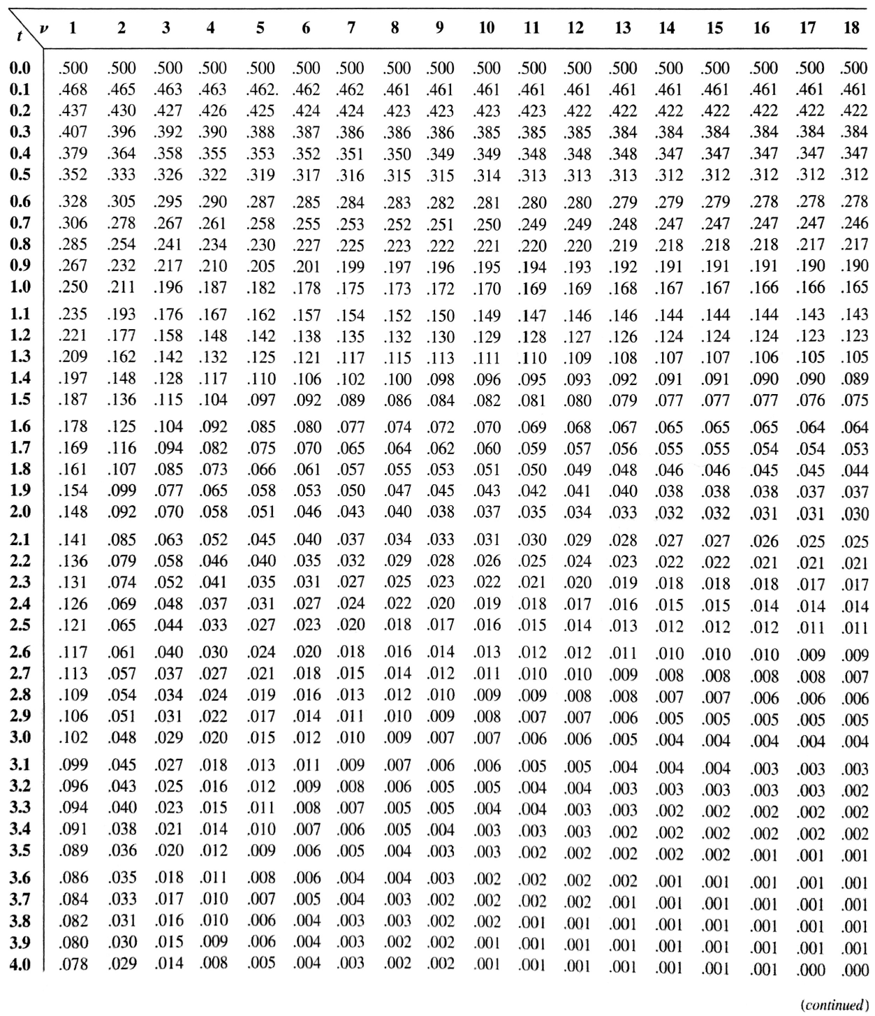
\[ \small{ \begin{aligned} &p\text{-value}\\ =\;&\text{P}(T_{v=15}< -1.801) \\ =\;&0.046 \end{aligned} } \]
Pooled t procedure
\[ \small{ T=\frac{\bar{X}-\bar{Y}-(\mu_X-\mu_Y)}{\sqrt{\frac{S_X^2}{m}+\frac{S_Y^2}{n}}},\;\;\;\; v=\frac{\big(\frac{S_X^2}{m}+\frac{S_Y^2}{n}\big)^2}{\frac{S_X^2/m}{m-1}+\frac{S_Y^2/n}{n-1}} } \]
If it’s reasonable to assume \(X\) and \(Y\) have (unknown but) equal variance (i.e., \(\sigma_X^2=\sigma_Y^2\)), we can simplify it to
\[ \small{ S_{\text{pooled}}^2=\frac{m-1}{m+n-2}S_X^2+\frac{n-1}{m+n-2}S_Y^2 } \]
\[ \small{ T=\frac{\bar{X}-\bar{Y}-(\mu_X-\mu_Y)}{S_{\text{pooled}}\sqrt{\frac{1}{m}+\frac{1}{n}}}}\;\text{ is approximately a $t$-distribution. } \]
\[ \small{ \text{with degree of freedom of $(m+n-2)$.} } \]
Paired t-test
- So far, we assumed \(X_1, X_2, \cdots, X_m\) and \(Y_1, Y_2, \cdots, Y_n\) are all independent.
- A group of people who eat fast food, and another group of people who don’t
- In many situations, there’s only one set of \(n\) individuals or objects, and we make two observations on each.
- Patient blood pressure before/after taking a drug
- Student test scores before/after a tutoring program
Assumptions
The data consists of \(n\) independently selected pairs
\[ (X_1, Y_1), (X_2, Y_2), \cdots, (X_n, Y_n) \]
Let \(D\) denotes the difference between the first and second observations within a pair.
\[ D_i = X_i-Y_i, \;\;\;\; i=1, 2, \cdots, n \]
\[ \mu_D=\text{E}[X-Y]=\mu_X-\mu_Y \]
Then we can do the one-sample test on the difference.
Paired t-test
\[ \begin{aligned} &H_0: \mu_D=0 \\ (1)\; &H_a: \mu_D \neq 0\;\;\;\;\color{gray}{\rightarrow\text{two-tailed}} \\ (2)\; &H_a: \mu_D>0\;\;\;\;\color{gray}{\rightarrow\text{one-tailed}} \\ (3)\; &H_a: \mu_D < 0\;\;\;\;\color{gray}{\rightarrow\text{one-tailed}} \\ \end{aligned} \]
\[ \text{The test statistic:}\;\;\;\;t=\frac{\bar{d}-0}{s_D/\sqrt{n}} \]
\[ \text{with a degree of freedom of $n-1$.} \]
Student test scores before/after a tutoring program
| Student | Before | After | Difference |
|---|---|---|---|
| 1 | 83 | 88 | 5 |
| 2 | 83 | 73 | -10 |
| 3 | 67 | 83 | 16 |
| 4 | 72 | 65 | -7 |
| 5 | 83 | 92 | 9 |
| 6 | 80 | 83 | 3 |
| 7 | 94 | 95 | 1 |
| 8 | 82 | 77 | -5 |
| 9 | 74 | 89 | 15 |
| 10 | 74 | 86 | 12 |
Is the tutoring program effective?
\[ \text{Difference: }[5, -10, 16, -7, 9, 3, 1, -5, 15, 12] \]
Let \(\mu_D\) denote the true average difference between the scores before and after the program.
\[ H_0: \mu_D=0, \;\;\;\;H_a: \mu > 0 \]
\[ n=10, \;\;\;\; \bar{d}=3.9, \;\;\;\; s_D=9.207 \]
\[ t=\frac{\bar{d}-0}{s_D/\sqrt{n}}=\frac{3.9}{9.207/\sqrt{10}}\approx 0.134 \]
\[ \text{with a degree of freedom of $n-1=9$.} \]
\[ \small{ \begin{aligned} &p\text{-value}\\ =\;&\text{P}(T_{v=9} > 0.134) \\ \approx\;& 0.461 \end{aligned} } \]