Procedures for constructing a CI
Suppose \(X_1, X_2, \cdots, X_n\) are i.i.d. normal, with unknown mean \(\theta\) and a known variance1 \(\sigma^2\).
\[
\hat{\Theta}_n=\frac{X_1+X_2+\cdots+X_n}{n}
\]
\[
\hat{\Theta}_n \sim \text{N}\bigg(\theta, \frac{\sigma^2}{n}\bigg)\;\;\rightarrow\;\;\frac{\hat{\Theta}_n-\theta}{\sigma/\sqrt{n}} \sim \text{N}(0, 1)
\]
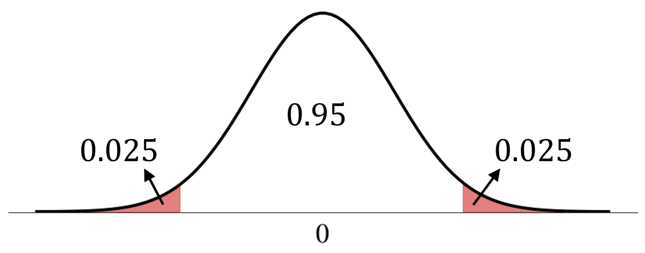
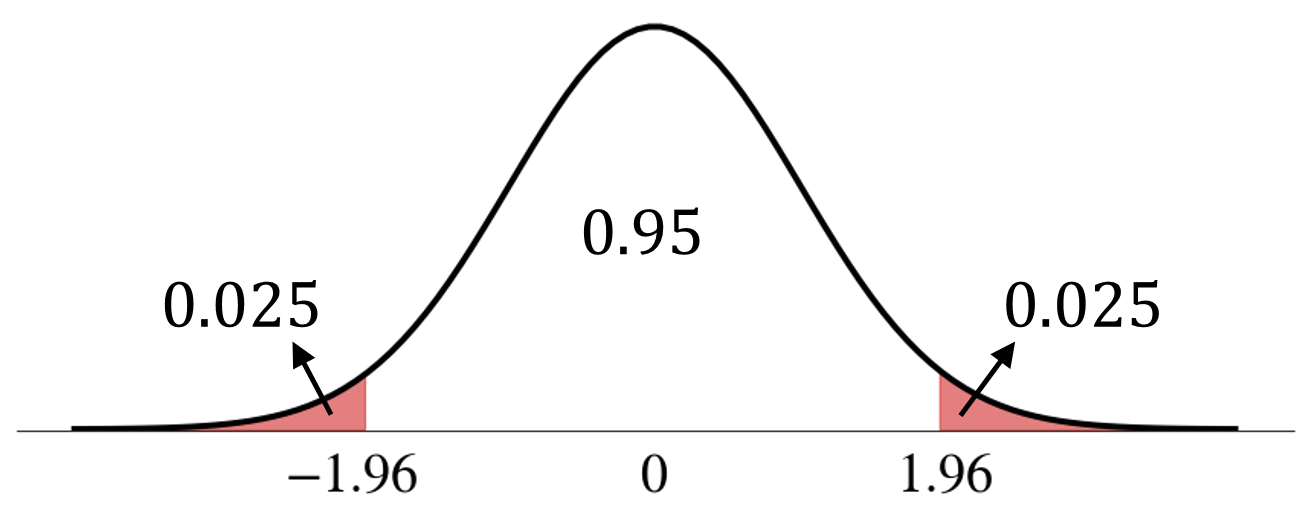
We want
\[
\text{P}\bigg(-1.96 < \frac{\hat{\Theta}_n-\theta}{\sigma/\sqrt{n}} < 1.96\bigg) = 0.95
\]
Multiply through by \(\sigma/\sqrt{n}\)
\[
\small{
\text{P}\bigg(-1.96 \cdot \frac{\sigma}{\sqrt{n}} < \hat{\Theta}_n-\theta < 1.96 \cdot \frac{\sigma}{\sqrt{n}}\bigg) = 0.95
}
\]
Subtract \(\hat{\Theta}_n\) from each term
\[
\small{
\text{P}\bigg(-\hat{\Theta}_n-1.96 \cdot \frac{\sigma}{\sqrt{n}} < -\theta < -\hat{\Theta}_n + 1.96 \cdot \frac{\sigma}{\sqrt{n}}\bigg) = 0.95
}
\]
Multiply through by \(-1\)
\[
\small{
\text{P}\bigg(\hat{\Theta}_n + 1.96 \cdot \frac{\sigma}{\sqrt{n}} > \theta > \hat{\Theta}_n - 1.96 \cdot \frac{\sigma}{\sqrt{n}}\bigg) = 0.95
}
\]
Rearange the sides.
\[
\text{P}\bigg(\hat{\Theta}_n - 1.96 \cdot \frac{\sigma}{\sqrt{n}} < \theta < \hat{\Theta}_n + 1.96 \cdot \frac{\sigma}{\sqrt{n}}\bigg) = 0.95
\]
This means that
\[
\bigg[\hat{\Theta}_n - 1.96 \cdot \frac{\sigma}{\sqrt{n}},\;\; \hat{\Theta}_n + 1.96 \cdot \frac{\sigma}{\sqrt{n}}\bigg]
\]
is a 95% confidence interval.
More compactly, it can be written as \(\hat{\Theta}_n \pm 1.96 \cdot \frac{\sigma}{\sqrt{n}}\)
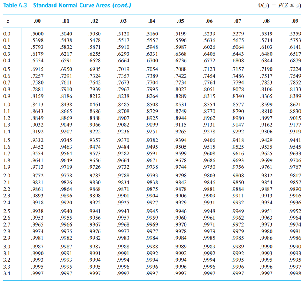
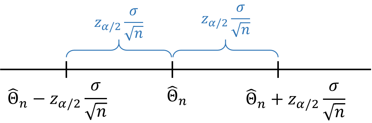
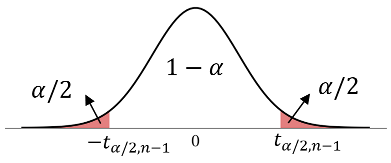
More generally, for a confidence level of \(1-\alpha\),
let \(z_{\frac{\alpha}{2}}\) be such that \(\Phi(z_{\frac{\alpha}{2}})=1-\frac{\alpha}{2}\).
![]()
\[
\small{
\text{P}\bigg(\hat{\Theta}_n - z_{\frac{\alpha}{2}} \frac{\sigma}{\sqrt{n}} < \theta < \hat{\Theta}_n + z_{\frac{\alpha}{2}} \frac{\sigma}{\sqrt{n}}\bigg) = 1-\alpha
}
\]
\[
\small{
\bigg[\hat{\Theta}_n - z_{\frac{\alpha}{2}} \frac{\sigma}{\sqrt{n}},\;\; \hat{\Theta}_n + z_{\frac{\alpha}{2}} \frac{\sigma}{\sqrt{n}}\bigg]}, \;\;\text{or }\;\; \hat{\Theta}_n \pm z_{\frac{\alpha}{2}} \frac{\sigma}{\sqrt{n}
}
\]
is a \((1-\alpha)\) confidence interval.
- It is a random interval centered at point estimate \(\hat{\Theta}_n\).
- The half-width of the CI is \(z_{\frac{\alpha}{2}} \frac{\sigma}{\sqrt{n}}\).
- The width of the CI indicates how precise the estimate is.
\[
\hat{\Theta}_n \pm z_{\alpha/2} \frac{\sigma}{\sqrt{n}}
\]
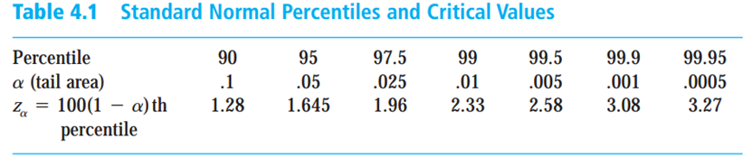
\[
\text{90% CI: }\;\;\;\; \hat{\Theta}_n \pm 1.645 \frac{\sigma}{\sqrt{n}}
\]
\[
\text{95% CI: }\;\;\;\; \hat{\Theta}_n \pm 1.96 \frac{\sigma}{\sqrt{n}}
\]
\[
\text{99% CI: }\;\;\;\; \hat{\Theta}_n \pm 2.58 \frac{\sigma}{\sqrt{n}}
\]
\[
\hat{\Theta}_n \pm z_{\frac{\alpha}{2}} \frac{\sigma}{\sqrt{n}}
\]
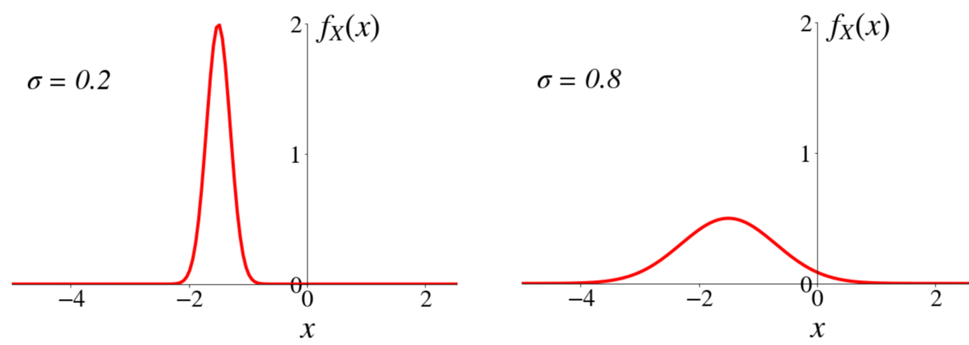
The half-width is proportional to \(\sigma\) (population standard deviation), the inherent variability of the thing we are trying to measure.
\[
\hat{\Theta}_n \pm z_{\frac{\alpha}{2}} \frac{\sigma}{\sqrt{n}}
\]
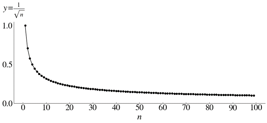
The half-width decreases as sample size \(n\) increases.
Sample size calculation
- We often have a desired precision (i.e., \(\pm 0.5\) hours) and a confidence level (e.g., 99%) for a confidence interval.
- Question: how many data points should we collect?
\[
\text{Half width:}\;\;d=z_{\frac{\alpha}{2}} \cdot \frac{\sigma}{\sqrt{n}}, \;\;\;\;\text{Solve for $n$.}
\]
The sample size needed for a desired half-width of \(d\) is
\[
n=\bigg(z_{\frac{\alpha}{2}} \cdot \frac{\sigma}{d}\bigg)^2
\]
Suppose \(X_1, X_2, \cdots, X_n\) are i.i.d. normal, with unknown mean \(\theta\) and known variance \(\sigma^2\).
\[
\small{
\text{Sample mean estimator:}\;\;\hat{\Theta}_n=\frac{X_1+X_2+\cdots+X_n}{n}
}
\]
\[
\small{
\text{var}\big(\hat{\Theta}_n\big)=\frac{\sigma^2}{n}, \;\;\;\;\sqrt{\text{var}\big(\hat{\Theta}_n\big)}=\frac{\sigma}{\sqrt{n}}
}
\]
The standard deviation of \(\hat{\Theta}_n\) is termed standard error.
\[
\hat{\Theta}_n \pm z_{\frac{\alpha}{2}} \frac{\sigma}{\sqrt{n}}
\]
The CI above can be expressed in words as
\[
\text{(point estimate)} \pm \text{($z$ critical value}) \cdot \text{(standard error)}
\]
Suppose \(X_1, X_2, \cdots, X_n\) are
- i.i.d. (not necessarily follow a normal distribution)
- with unknown mean \(\theta\) and known variance \(\sigma^2\)
\[
\small{\text{Sample mean estimator:}\;\;\hat{\Theta}_n=\frac{X_1+X_2+\cdots+X_n}{n}}
\]
If \(n\) is sufficiently large, what does the CLT tell us?
\[
\small{
\begin{aligned}
\hat{\Theta}_n \;&\text{ is approximately } \text{N}\bigg(\theta, \frac{\sigma^2}{n}\bigg) \\
\frac{\hat{\Theta}_n-\theta}{\sigma/\sqrt{n}} \;&\text{ is approximately } \text{N}(0, 1) \\
\end{aligned}
}
\]
Procedures for constructing a CI
We can proceed exactly as in the previous case.
![]()
\[
\text{P}\bigg(-z_{\frac{\alpha}{2}} < \frac{\hat{\Theta}_n-\theta}{\sigma/\sqrt{n}} < z_{\frac{\alpha}{2}}\bigg) \approx 1-\alpha \;\;\;\color{gray}{\rightarrow \text{by CLT}}
\]
\[
\text{P}\bigg(\hat{\Theta}_n - z_{\frac{\alpha}{2}} \frac{\sigma}{\sqrt{n}} < \theta < \hat{\Theta}_n + z_{\frac{\alpha}{2}} \frac{\sigma}{\sqrt{n}}\bigg) \approx 1-\alpha
\]
What if we don’t know \(\sigma^2\)?
Suppose \(X_1, X_2, \cdots, X_n\) are i.i.d. with unknown mean \(\theta\) and unknown variance \(\sigma^2\).
\[
\small{
\text{Sample mean estimator:}\;\;\hat{\Theta}_n=\frac{X_1+X_2+\cdots+X_n}{n}
}
\]
We can estimate the population variance \(\sigma^2\) with
\[
\small{
\text{Sample variance estimator:}\;\;\hat{S}_n^2=\frac{\sum\big(X_i - \hat{\Theta}_n\big)^2}{n-1}
}
\]
\[
\small{
\frac{\hat{\Theta}_n-\theta}{\sigma/\sqrt{n}} \sim \text{N}(0, 1), \; \text{if $X_i$ is normally distributed.}
}
\]
\[
\small{
\frac{\hat{\Theta}_n-\theta}{\sigma/\sqrt{n}} \text{ is approximately } \text{N}(0, 1), \; \text{if $X_i$ is not normal, but $n$ is large.}
}
\]
Once we replace \(\sigma\) with \(\hat{S}_n\), we have
\[
\small{
\frac{\hat{\Theta}_n-\theta}{\hat{S}_n/\sqrt{n}}
}
\]
\[
\small{
\frac{\hat{\Theta}_n-\theta}{\hat{S}_n/\sqrt{n}} \text{ is approximately } \text{N}(0, 1), \; \text{if $n$ is sufficiently large.}
}
\]
If \(n\) is sufficiently large,
\[
\small{
\text{P}\bigg(-z_{\frac{\alpha}{2}} < \frac{\hat{\Theta}_n-\theta}{\hat{S}_n/\sqrt{n}} < z_{\frac{\alpha}{2}}\bigg) \approx 1-\alpha
}
\]
Generally speaking, \(n>40\) would be sufficient.
\[
\small{
\hat{\Theta}_n \pm z_{\frac{\alpha}{2}} \frac{\hat{S}_n}{\sqrt{n}}
}
\]
is a CI for \(\theta\) with confidence level approximately \(1-\alpha\).
\[
\small{
\text{(point estimate)} \pm \text{($z$ critical value)} \cdot \text{(estimated standard error)}
}
\]
What if the sample size \(n\) is small?
Suppose \(X_1, X_2, \cdots, X_n\) are i.i.d. normal with unknown mean \(\theta\) and unknown variance \(\sigma^2\).
\[
\small{
\text{Sample mean estimator:}\;\;\hat{\Theta}_n=\frac{X_1+X_2+\cdots+X_n}{n}
}
\]
\[
\small{
T_n=\frac{\hat{\Theta}_n-\theta}{\hat{S}_n/\sqrt{n}}
}
\]
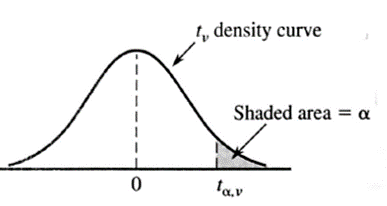
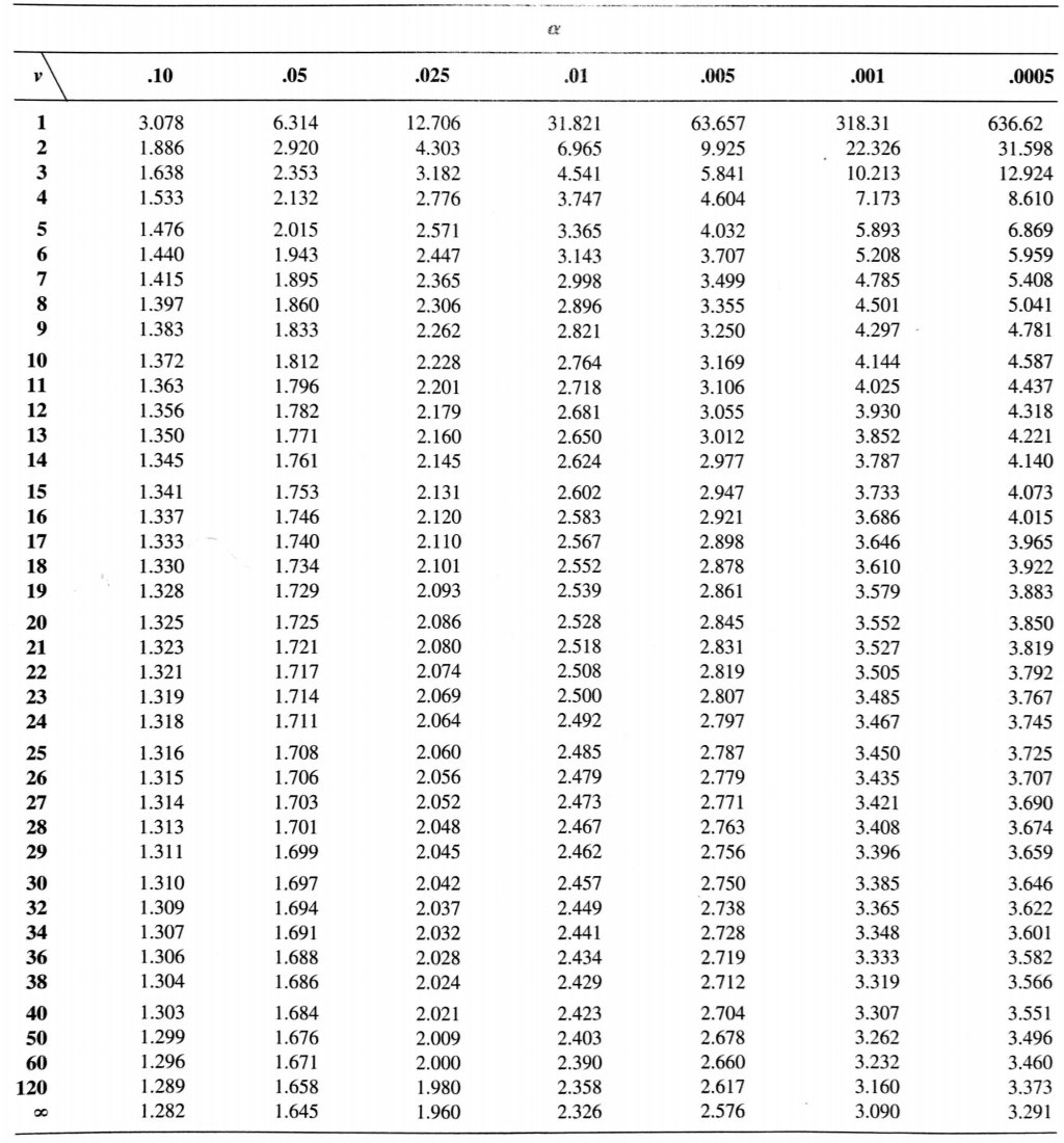
has a probability distribution called a t-distribution with \(v=n-1\) degrees of freedom.
\[
\small{
t\text{-distribution:}\;\;\;T_n=\frac{\hat{\Theta}_n-\theta}{\hat{S}_n/\sqrt{n}}
}
\]
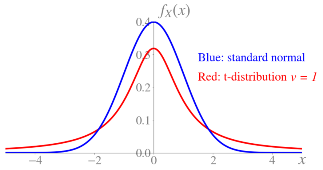
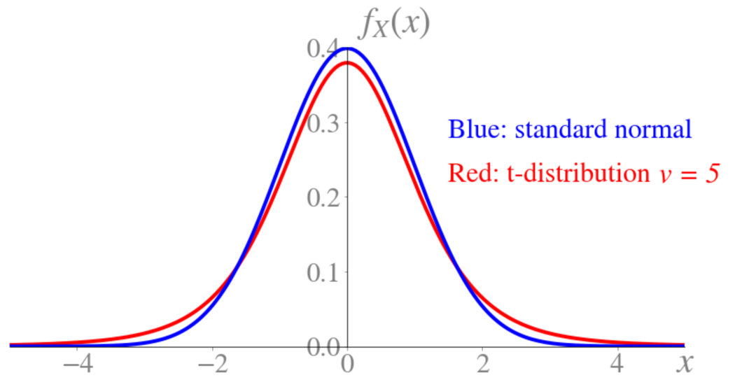
t-distribution
- Symmetric
- Bell-shaped
- More spread out than \(N(0, 1)\)
- Approaches \(N(0, 1)\) as \(v\rightarrow +\infty\)