5.1 Joint & marginal PMF

Joint PMF

Randomly select a person on campus and record their age and number of credit cards they own.

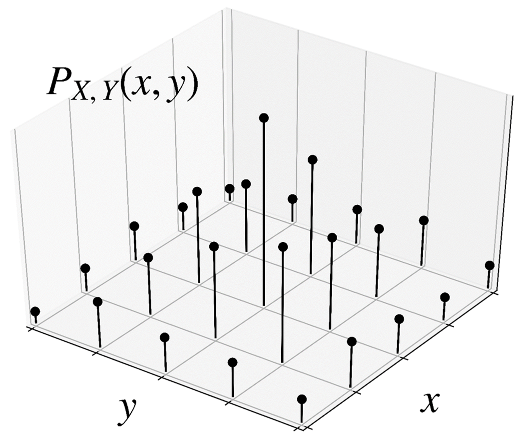
Definition: Two discrete RV $X$ and $Y$ from the same experiment. $(x, y)$ is a pair of possible values of $X$ and $Y$.

The joint PMF of $X$ and $Y$ is defined as

\[ p_{X, Y}(x, y) \stackrel{\text{def}}{=} \text{P}\big(\{X=x\} \cap \{Y=y\}\big) \]

For simplicity, we often use the abbreviated notation.

\[ p_{X, Y}(x, y) \stackrel{\text{def}}{=} \text{P}(X=x, Y=y) \]

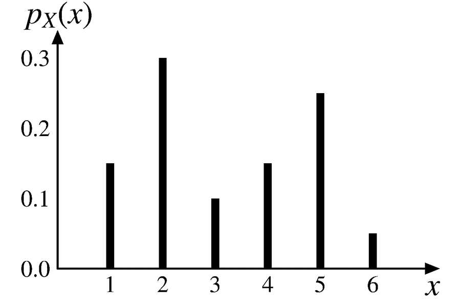
Recall the PMF of a single random variable is defined as

\[ p_{X}(x) \stackrel{\text{def}}{=} \text{P}(X=x) \]

\[ p_{X, Y}(x, y) \stackrel{\text{def}}{=} \text{P}(X=x, Y=y) \]

We randomly sample an adult from the MI population.
- $X$: whether they are a current smoker
- $Y$: whether they will develop lung cancer at some point
Suppose the joint PMF is as follows.

$Y=0$ $Y=1$

$X=0$ $72\%$ $3\%$

$X=1$ $20\%$ $5\%$

	\(Y=0\)	\(Y=1\)
\(X=0\)	\(72\%\)	\(3\%\)
\(X=1\)	\(20\%\)	\(5\%\)

PMF of a single discrete RV $X$

\[ p_X(x) \geq 0, \;\; \text{for all $x$.} \]

Joint PMF of two discrete RVs $X$ and $Y$

\[ p_{X, Y}(x, y) \geq 0, \;\;\;\; \text{for all $x$ and $y$.} \]

For a single discrete RV $X$, we have

\[ \sum_x p_X(x)=1 \]

Joint PMF of two discrete RVs $X$ and $Y$

\[ \sum_x\sum_y p_{X, Y}(x, y)=1 \]

	$Y=0$	$Y=1$
$X=0$	$72\%$	$3\%$
$X=1$	$20\%$	$5\%$

The CDF of a RV $X$ is (always) defined by

\[ F_X(x) \stackrel{\text{def}}{=} \text{P}(X \leq x), \;\; \text{for all $x$.} \]

The joint CDF of two RVs $X$ and $Y$ is defined by

\[ F_{X, Y}(x, y) \stackrel{\text{def}}{=} \text{P}(X \leq x, Y \leq y), \;\;\;\;\;\text{for all $x$ and $y$.} \]

Joint CDFs are generally harder to work with than joint PMFs.

For this reason, we will mainly stick with joint PMFs.

$A$: the set of all pairs $(x, y)$ that have a certain property.

\[ \text{P}\big((X, Y) \in A\big)=\sum_{(x, y) \in A}p_{X, Y}(x, y) \]

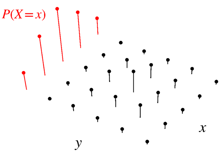
We can calculate the PMF of $X$ using

\[ \small{ p_X(x)=\text{P}(X=x)=\sum_\color{blue}{y} \text{P}(X=x, Y=y) =\sum_\color{blue}{y} p_{X, Y}(x, y) } \]

We refer to $p_X(x)$ as the marginal PMF of $X$.

Similarly, we can calculate the PMF of $Y$ using

\[ \small{ p_Y(y)=\text{P}(Y=y)=\sum_\color{red}{x} \text{P}(X=x, Y=y)=\sum_\color{red}{x} p_{X, Y}(x, y) } \]

We refer to $p_Y(y)$ as the marginal PMF of $Y$.

We randomly sample an adult from the MI population.
- $X$: whether they are a current smoker
- $Y$: whether they will develop lung cancer at some point
Suppose the joint PMF is as follows.

$Y=0$ $Y=1$

$X=0$ $72\%$ $3\%$

$X=1$ $20\%$ $5\%$
What are the marginal PMFs of $X$ and $Y$?