Normal distribution
A continuous RV \(X\) is normal if it has a PDF:
\[
f_X(x)=\frac{1}{\sigma\sqrt{2\pi}}e^{-\frac{1}{2}(\frac{x-\mu}{\sigma})^2}
\]
\[
\text{where } \mu \text{ and } \sigma \text{ are its two parameters } (\sigma >0).
\]
\[
X \sim \text{N}(\mu, \sigma^2)
\]
Normal distribution
\[
\begin{aligned}
X &\sim \text{N}(\mu, \sigma^2) \\
\\
f_X(x)&=\frac{1}{\sigma\sqrt{2\pi}}e^{-\frac{1}{2}(\frac{x-\mu}{\sigma})^2} \\
\\
\text{E}[X]&=\mu \\
\\
\text{var}(X)&=\sigma^2 \\
\end{aligned}
\]
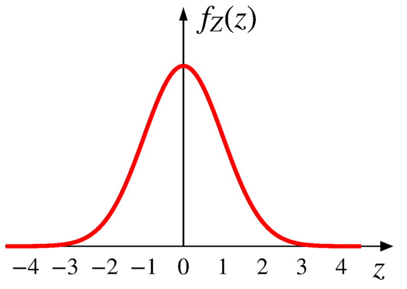
First, we show that the expected value of a standard normal RV \(Z \sim \text{N}(0, 1)\) is zero.
\[
\begin{aligned}
f_Z(z)&=\frac{1}{\sqrt{2\pi}}e^{-\frac{z^2}{2}} \\
\\
\text{E}[Z]&=\int_{-\infty}^{+\infty}z(\frac{1}{\sqrt{2\pi}}e^{-\frac{z^2}{2}})dz=0 \\
\end{aligned}
\]
The integration above is 0 as for any odd function \(g(x)\) (i.e., \(g(-x)=-g(x)\) ), we have \(\int_{-a}^a g(x)dx=0\) .
Let
\[Z=\frac{X-\mu}{\sigma} \;\;\;\;(\text{or } X=\sigma Z+\mu)\]
We have
\[f_X(x)=\frac{1}{\sigma\sqrt{2\pi}}e^{-\frac{1}{2}(\frac{x-\mu}{\sigma})^2}\]
\[X \sim \text{N}(\mu, \sigma^2)\]
\[\text{E}[X]=\text{E}[\sigma Z+\mu]=\sigma\text{E}[Z]+\mu=\sigma\cdot 0+\mu=\mu\]
We can also prove for \(Z \sim \text{N}(0, 1)\) , \(\text{var}(Z)=1\) .
\[
\begin{aligned}
\text{var}(Z)&=\text{E}\big[Z^2\big]-\big(\text{E}[Z]\big)^2 \\
\\
&=\int_{-\infty}^{+\infty}z^2(\frac{1}{\sqrt{2\pi}}e^{-\frac{z^2}{2}})dz \\
\\
&=1 \;\;\;\;\color{gray}{\rightarrow\text{we will skip the proof of this part.}}
\end{aligned}
\]
Then we have \[\text{var}(X)=\text{var}(\sigma Z+\mu)=\sigma^2\text{var}(Z)=\sigma^2 \cdot 1 = \sigma^2\]
Properties
Normality is preserved by linear transformations.
If
\[
X \sim \text{N}(\mu, \sigma^2)
\]
and
\[
Y=aX+b, \;\; \text{for any constants } a \;(\neq0) \text{ and $b$.}
\]
we have
\[
Y \sim \text{N}(a\mu+b, a^2\sigma^2)
\]
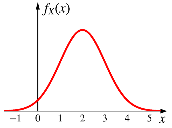
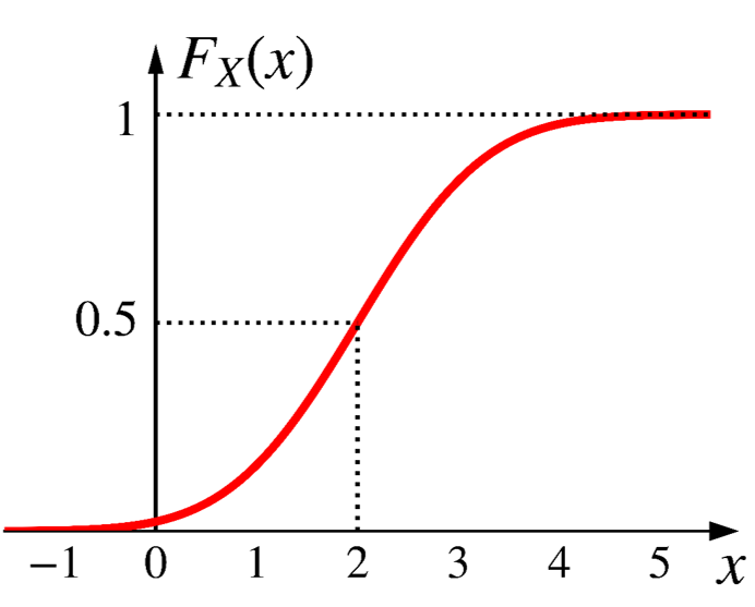
CDF of normal distribution
\[
X \sim \text{N}(2, 1)
\]
CDF of normal distribution
\[
\begin{aligned}
F_X(x)&=\text{P}(X \leq x) \\
\\
&=\int_{-\infty}^x \frac{1}{\sigma\sqrt{2\pi}}e^{-\frac{1}{2}\big(\frac{t-\mu}{\sigma}\big)^2}dt \\
\\
&=\frac{1}{\sigma\sqrt{2\pi}}\int_{-\infty}^x e^{-\frac{1}{2}\big(\frac{t-\mu}{\sigma}\big)^2}dt \\
\end{aligned}
\]
Unfortunately, there is no closed-form expression for the integration above.
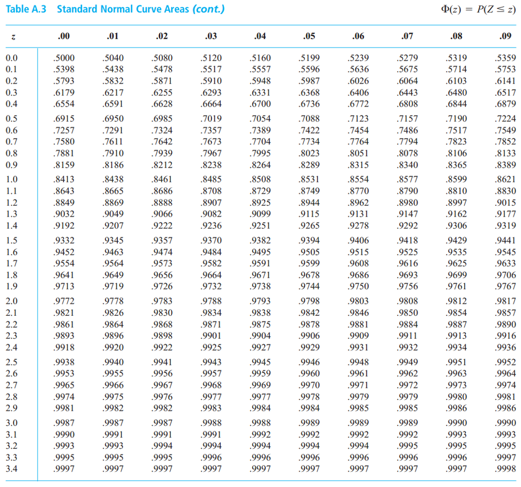
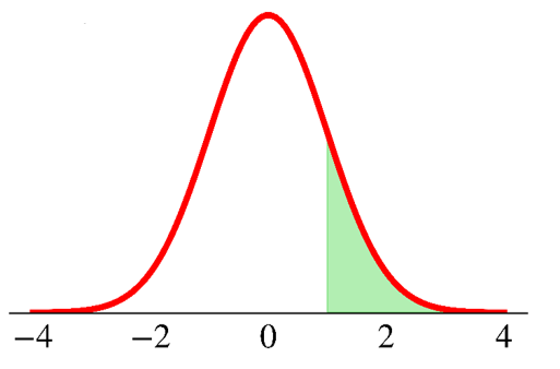
CDF of standard normal distribution
\[
F_Z(z)=\Phi(z)=\text{P}(Z \leq z)=\frac{1}{\sqrt{2\pi}}\int_{-\infty}^z e^{-\frac{t^2}{2}}dt
\]
Standard normal table (or Z table)
The table only contains values of \(\Phi(z)\) for \(z \geq 0\) .
What if \(z < 0\) ?
Exercise
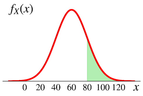
Assume the annual snowfall in Dearborn follows a normal distribution with
a mean of 60 inches
a standard deviation of 20 inches
What is the probability this year has 80+ inches snow?
\[
X \sim \text{N}\big(\mu, \sigma^2\big)
\]
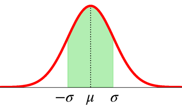
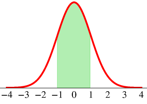
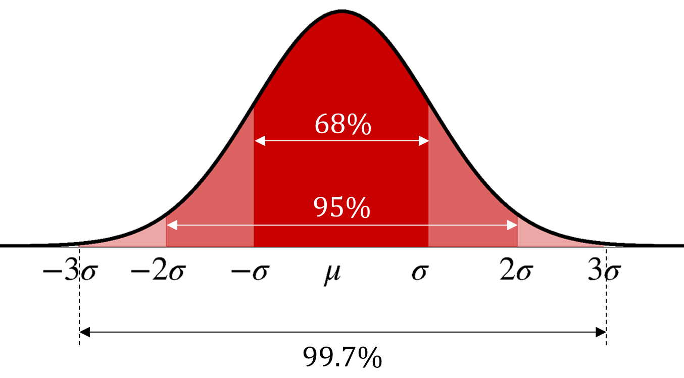
What is the probability that \(X\) takes values within one standard deviation from its mean?
\[
\text{P}(\mu - \sigma < X < \mu + \sigma) = \;?
\]
\[
X \sim \text{N}\big(\mu, \sigma^2\big)
\]
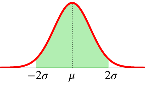
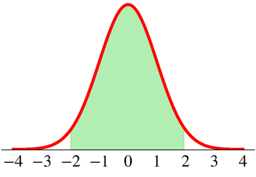
What is the probability that \(X\) takes values within two standard deviation from its mean?
\[
\text{P}(\mu - 2\sigma < X < \mu + 2\sigma) = \;?
\]
\[
X \sim \text{N}\big(\mu, \sigma^2\big)
\]
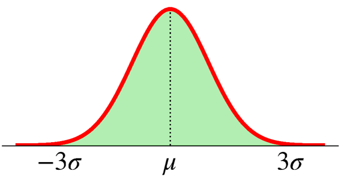
What is the probability that \(X\) takes values within three standard deviation from its mean?
\[
\text{P}(-3\sigma < X < 3\sigma) = \;?
\]
68-95-99.7 rule
\[
X \sim \text{N}\big(\mu, \sigma^2\big)
\]
Six Sigma
\[
\text{P}(\mu - 6\sigma < X < \mu + 6 \sigma)=99.99966\%
\]
The procedure to get the normal CDF
Standardize \(X\) to obtain the standard normal \(Z\) \[\small{Z=\frac{X-\mu}{\sigma}}\]
Obtain the CDF value from the \(Z\) table
\[
\small{
\begin{aligned}
\text{P}(X < x)&=\text{P}\bigg(\frac{X-\mu}{\sigma} < \frac{x-\mu}{\sigma}\bigg)\\
&=\text{P}\bigg(Z < \frac{x-\mu}{\sigma}\bigg)
=\Phi\bigg(\frac{x-\mu}{\sigma}\bigg) \\
\end{aligned}
}
\]
Getting normal CDF in Python
Go to Google Colab and sign in. Open a new notebook.
# get the CDF of a standard normal distribution from scipy import stats= 0 )
How about \(F_X(x=0)=\text{P}(X \leq 0)\) where \(X \sim \text{N}(1, 3^2)\) ?
# get the CDF of a non-standard normal distribution = 0 , loc= 1 , scale= 3 )
Mixed random variables
As a final note to Chapter 3 & 4, a random variable could be a mixture of both discrete & continuous.
Consider the following game of tossing a coin
If it lands on heads, you get $10.
If it lands on tails, you get $ amount of \(\text{unif}(5, 15)\) .