3.8 Binomial distribution

• Toss a coin for \(n\) times. At each toss,
  • it lands on a heads with probability of \(p\)
  • it lands on a tails with probability of \(1-p\).

Let \(X\) represents the number of heads we get after \(n\) tosses.

We refer to \(X\) as a binomial RV with parameters \(n\) and \(p\).

Or simply

\[ X \sim \text{bin}(n, p) \]

Toss a coin for 3 times. What’s the prob. to get exact 2 heads?

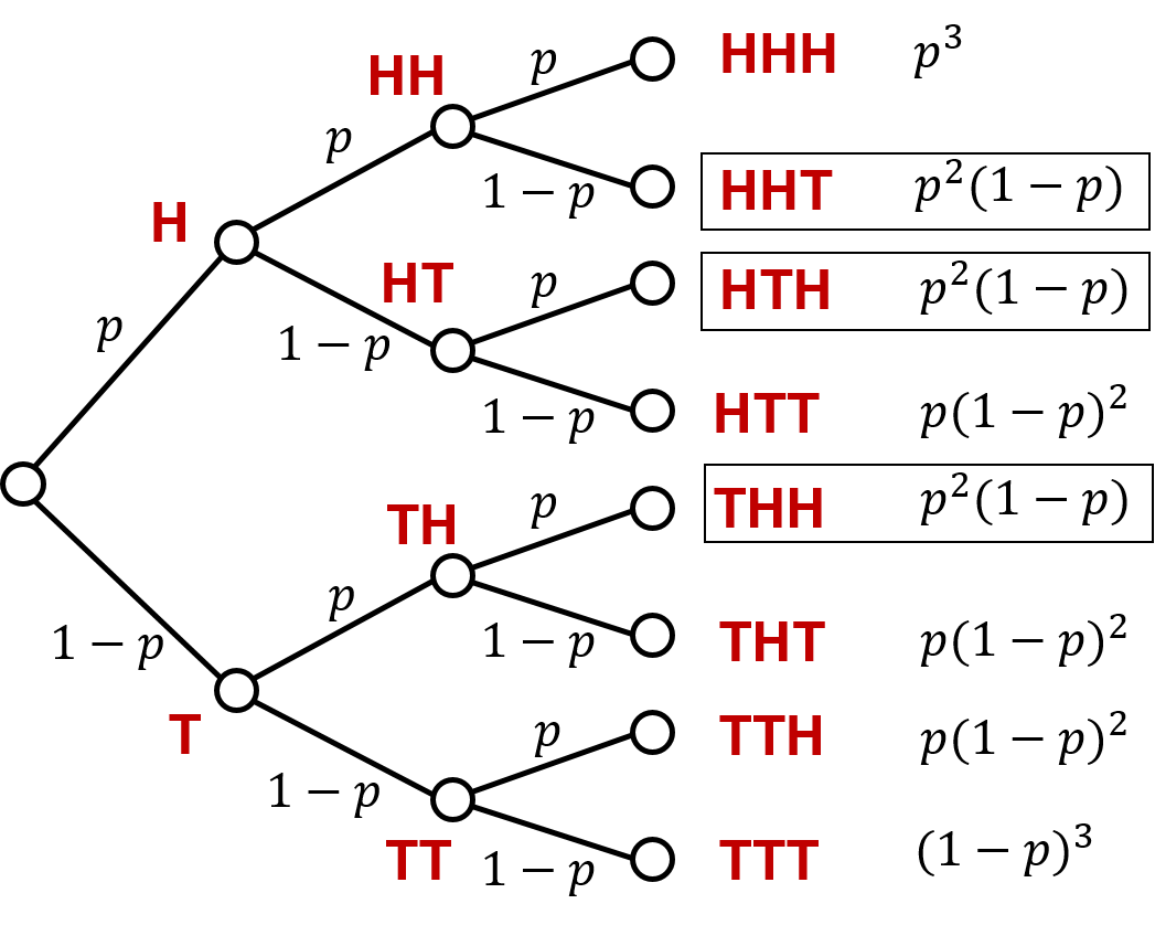
\[ \small{\text{P}(\text{getting exact 2 heads})={3 \choose 2}p^2(1-p)} \]

Probability mass function (PMF)

\(X\): the number of heads we get after \(n\) tosses.

\[ X \sim \text{bin}(n, p) \]

\[ p_X(k)=\text{P}(X=k) ={n \choose k}p^k(1-p)^{n-k} \;\;\text{for } k=0, 1, 2, \cdots, n. \]

Why it is called binomial?

\[ p_X(k)=\text{P}(X=k) ={n \choose k}p^k(1-p)^{n-k} \;\;\text{for } k=0, 1, 2, \cdots, n. \]

It has the same format as the binomial expansion terms in algebra:

\[ (x+y)^n=\sum_{k=0}^n {n \choose k}x^k y^{n-k} \]

where \({n \choose k}\) is called the binomial coefficient.

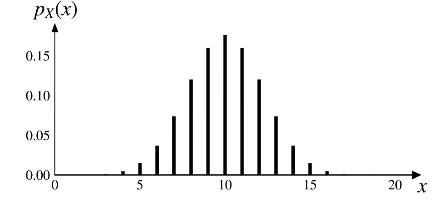
\(\text{bin}(20, \color{red}{0.5})\)

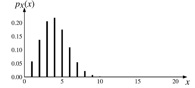
\(\text{bin}(20, \color{red}{0.2})\)

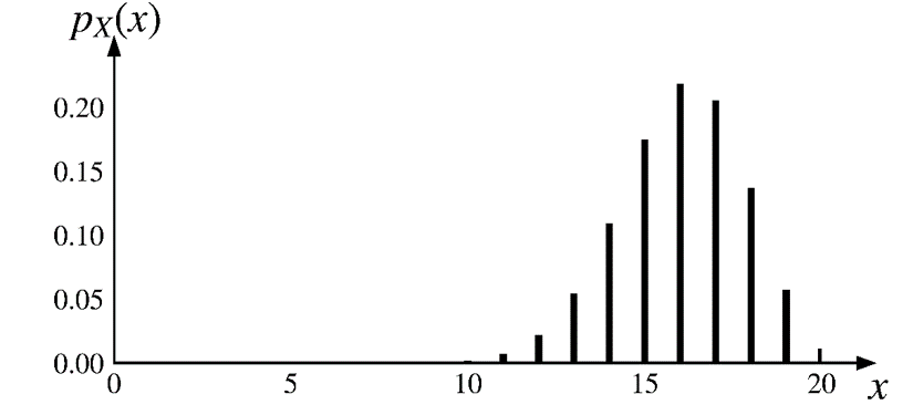
\(\text{bin}(20, \color{red}{0.8})\)

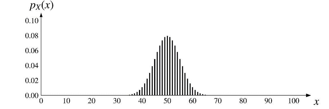
\(\text{bin}(100, \color{red}{0.5})\)

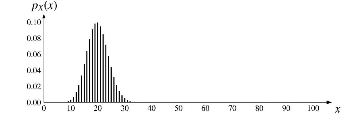
\(\text{bin}(100, \color{red}{0.2})\)

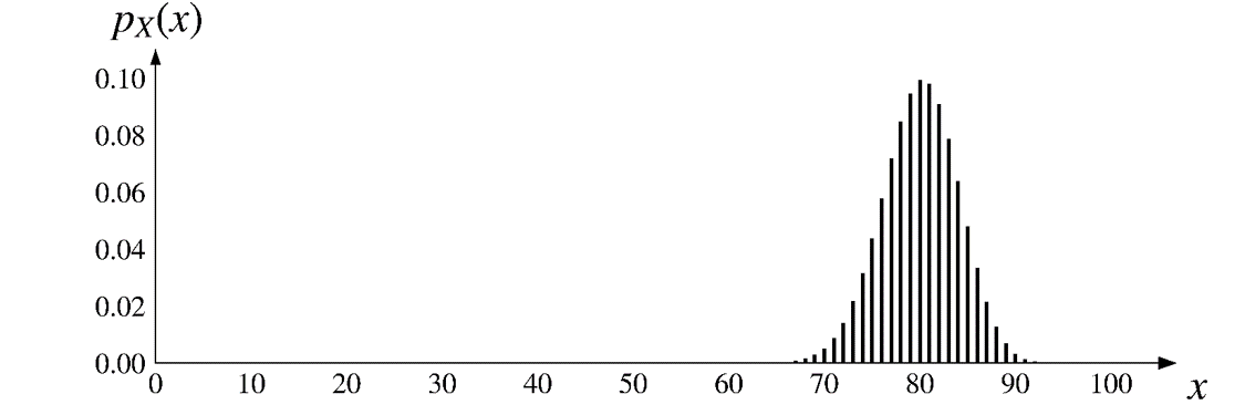
\(\text{bin}(100, \color{red}{0.8})\)

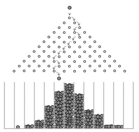
Interactive visualization

Galton Board

Expected value

\[ p_X(k)=\text{P}(X=k) ={n \choose k}p^k(1-p)^{n-k} \;\;\text{for } k=0, 1, 2, \cdots, n. \]

\[ \text{E}[X]=\sum_{k=0}^n \bigg[k \cdot {n \choose k}p^k(1-p)^{n-k}\bigg] \]

A shortcut to find the expected value of a binomial RV

\[ \small{ X \sim \text{Bernoulli}(p), \;\;\;\; p_X(x) = \begin{cases} p, & \text{if $x = 1$,} \\ 1-p, & \text{if $x = 0$.} \\ \end{cases} } \]

A binomial RV is the sum of \(n\) independent & identically distributed (i.i.d.) Bernoulli RVs.

\[ Y=X_1+X_2+\cdots+X_n \]

\[ \begin{aligned} X_i \text{'s are i.i.d.} &\sim \text{Bernoulli}(p) \\ \\ Y&=X_1+X_2+\cdots+X_n \\ \\ Y &\sim \text{bin}(n, p) \\ \\ \text{E}[Y] &= \text{E}[X_1+X_2+\cdots+X_n] \end{aligned} \]

Linearity of the expected value

For any given constants \(a\) and \(b\), we have

\[ \text{E}[aX+b]=a \text{E}[X] + b \]

Given any two random variables \(X\) and \(Y\), we have

\[ \text{E}[X+Y]=\text{E}[X] + \text{E}[Y] \]

Note it does not require \(X\) and \(Y\) to be independent.

More generally, given any \(n\) RVs \(X_1, X_2, \cdots, X_n\)

\[ \text{E}[X_1+X_2+\cdots+X_n] = \text{E}[X_1] + \text{E}[X_2]+\cdots+\text{E}[X_n] \]

Lastly,

\[ \begin{aligned} \text{E}[Y] &= \text{E}[X_1+X_2+\cdots+X_n] \\ \\ &=\text{E}[X_1] + \text{E}[X_2]+\cdots+\text{E}[X_n] \\ \\ &=p + p+\cdots+p \\ \\ &= np \end{aligned} \]

If two RVs \(X\) and \(Y\) are independent, we have

\[ \text{var}(X+Y)=\text{var}(X) + \text{var}(Y) \]

More generally, if \(n\) RVs \(X_1, X_2, \cdots, X_n\) are independent,

\[ \begin{aligned} &\text{var}(X_1+X_2+\cdots+X_n) \\ =\;&\text{var}(X_1) + \text{var}(X_2)+\cdots+\text{var}(X_n) \\ \end{aligned} \]

Lastly, we can computer the variance of a binomial RV \(Y\) as

\[ \begin{aligned} \text{var}(Y) &= \text{var}(X_1+X_2+\cdots+X_n) \\ \\ &=\text{var}(X_1) + \text{var}(X_2)+\cdots+\text{var}(X_n) \\ \\ &=p(1-p) + p(1-p)+\cdots+p(1-p) \\ \\ &= np(1-p) \end{aligned} \]