Bad idea.
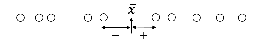
We can show that the sum of all deviations from the sample mean is always zero.
\[(x_1-\bar{x}) + (x_2-\bar{x}) + \cdots + (x_n-\bar{x})=0\]
Or, \[\sum_{i=1}^{n}(x_i-\bar{x})=0\]
If we cannot use the average deviation as a metric for variability, what can we do then?
One solution is to use the absolute deviations. \[\frac{1}{n}\bigg[|x_1-\bar{x}| + |x_2-\bar{x}| + \cdots + |x_n-\bar{x}|\bigg]\]
However, absolute values would lead to a number of mathematical difficulties later on.
The squared deviations is the preferred approach. \[(x_1-\bar{x})^2, \;(x_2-\bar{x})^2, \;\cdots, \;(x_n-\bar{x})^2\]
Sample variance
\[\begin{aligned}
s^2 &= \frac{(x_1-\bar{x})^2 + (x_2-\bar{x})^2 + \cdots + (x_n-\bar{x})^2}{n-1} \\
\\
&= \frac{\displaystyle\sum_{i=1}^{n}(x_i-\bar{x})^2}{n-1}
\end{aligned}\]
Why divided by \((n-1)\) instead of \(n\)?
- Degree of freedom: The number of values in a calculation that are free to vary.
- Pick any three numbers and calculate the mean.
- Now we add some constraints:
- The numbers have to add up to 20.
- The first two numbers have to add up to 10.
\[
s^2 = \frac{(x_1-\bar{x})^2 + (x_2-\bar{x})^2 + \cdots + (x_n-\bar{x})^2}{n-1}
\]
Are there any constraints when we calculate the sample variance?
Heights (in feet) of 216 volcanoes:
\[19882, 19728, 19335, 19287, \cdots, 617, 555, 529, 242\]
Sample mean:
\[\bar{x}=7047.6 \text{ feet}\]
Sample variance:
\[s^2 = \frac{\sum_{i=1}^{n}(x_i-\bar{x})^2}{n-1}=18,507,834 \text{ feet}^2\]
\[s^2 = \frac{\sum_{i=1}^{n}(x_i-\bar{x})^2}{n-1}=18,507,834 \text{ feet}^2\]
The sample standard deviation \(s\), is given by
\[ s = \sqrt{s^2} = \sqrt{\frac{\sum_{i=1}^{n}(x_i-\bar{x})^2}{n-1}}=4302.1 \text{ (ft})\]
Property I
\(x_1, x_2, \cdots, x_n\) are sample data. \(c\) is any constant.
\[\text{If }\; y_1=x_1+c, \;y_2=x_2+c, \;\cdots, \;y_n=x_n+c\]
\[\begin{aligned}
\text{then }\; s_y^2&=s_x^2 \\
(\text{or }s_y&=s_x)
\end{aligned}\]
Intuition: Adding a constant to the data shifts the distribution right or left without changing its shape, and thus its spread.
Property II
\(x_1, x_2, \cdots, x_n\) are sample data and \(c\) is any constant.
\[\text{If }\; y_1=cx_1, \;y_2=cx_2, \;\cdots, \;y_n=cx_n\]
\[
\begin{aligned}
\text{then } \; s_y^2&=c^2s_x^2 \\
(\text{or }s_y&=cs_x)
\end{aligned}
\]
Intuition: Multiplying a constant to the data changes its shape, and thus its spread.
Descriptive statistics with Python
Go to Google Colab and sign in. Open a new notebook.
ages = [12, 34, 14, 5, 44, 28, 22, 19, 36, 25]

mean = sum(ages) / len(ages)

squared_dev = [(x-mean)**2 for x in ages]

var = sum(squared_dev) / (len(ages) - 1)
print(var)

print(var**0.5)
import statistics
print(statistics.variance(ages))
print(statistics.stdev(ages))
Descriptive statistics with Python
We use the pandas library.
import pandas
url = "https://imse317.github.io/lecture-slides/ch01/data/bank.csv"
bank = pandas.read_csv(url)
bank.head()
print(bank["age"].var())
print(bank["age"].std())